
Transmittance spectra (.sp)
Upload one or more .sp files written by UV WinLab: the server checks them,
decodes them and, for each one, returns in a tab of its own the chart of
transmittance versus wavelength and the summary table — sample, instrument and
method recorded in the file, spectral data, derived quantities and measurement quality.
With two or more files, Show together puts all the spectra in a single chart, one
series per file that the legend switches on and off, and leaves the tables in the tabs.
How to read the results is explained in the Use tab.
Files to analyse
You can also drag the files onto this box. At most 50 files of 300 kB at a time.
This tab describes the instrument, the format of the files it produces and the software that drives it. The information on instrument and software comes from the official PerkinElmer documentation, listed at the end; where the documents disagree, or where a value was derived from the files rather than read in a manual, this is stated.
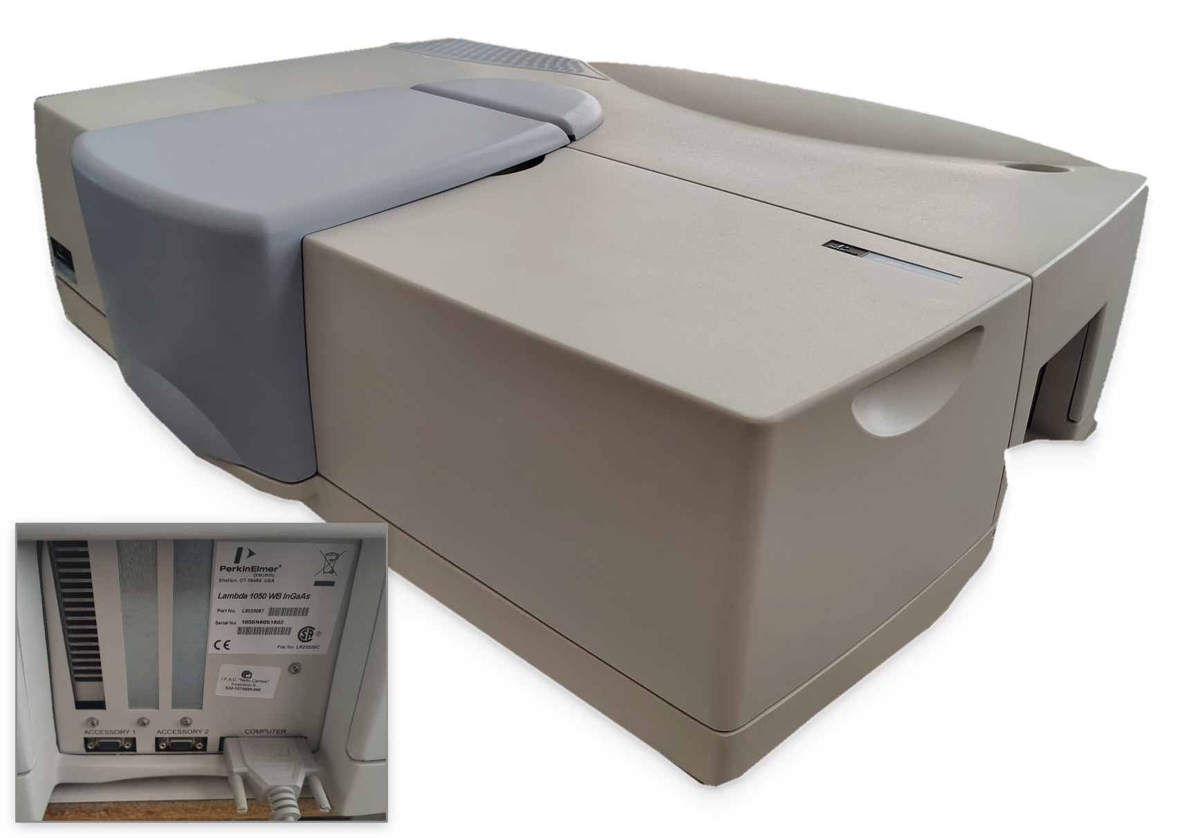
The PerkinElmer LAMBDA 1050 spectrophotometer
It is a double-beam, double-monochromator UV/Vis/NIR spectrophotometer of
PerkinElmer's "high-performance" family (LAMBDA 650, 750, 850, 950, 1050). The one that
produced the files of the technical report has serial number 1050N8051802 and,
according to the accessory list recorded in the files, motorised attenuators on both beams
(RBeamAtt, SBeamAtt) and the three-detector module with a
wide-band InGaAs (TDS WB InGaAs Detector). The hardware guide says that the
optics of the 1050 are those of the LAMBDA 950 with three differences: a mirror that doubles
the light of the halogen lamp, internal attenuators of 0 %, 0.1 %, 1 % and 100 % (the
950 has 10 % instead of 0.1 %) and the three-detector module fitted as standard.
| Part | Declared characteristics |
|---|---|
| Monochromators | all-reflecting double monochromator, Littrow mounting, holographic gratings: 1440 lines/mm blazed at 240 nm for UV/Vis and 360 lines/mm blazed at 1100 nm for the NIR. The grating changes during the scan, by default at 860.8 nm |
| Sources | deuterium lamp and tungsten-halogen lamp, pre-aligned; lamp change by default at 319.2 nm, not to be moved outside 300–350 nm. Recommended warm-up: about one hour |
| Detectors | R6872 photomultiplier from 175 to 860 nm; Peltier-cooled InGaAs, narrow-band (860–1800 nm) or wide-band (860–2500 nm); lead sulphide (PbS) up to 3300 nm. Detector changes by default at 860.8 nm and 1800.8 nm |
| Chopper | dark / sample / dark / reference cycle at more than 46 Hz: the dark signal is measured and subtracted at every cycle |
| Slits | UV/Vis from 0.05 to 5 nm, NIR from 0.2 to 20 nm; in the NIR also servo, which adjusts them during the scan according to the energy on the reference beam |
| Beam | about 12 mm high at the sample plane, about 4.5 mm wide with a 5 nm slit; the common beam mask reduces its height from 11.7 mm to zero in 50 steps. The two beams run 90 mm above the compartment floor, 120 mm apart |
| Range | 175–3300 nm (below 185 nm with nitrogen purge) |
| Stray light | 0.00007 %T at 220 nm (NaI), 340 and 370 nm (NaNO2); 0.00040 %T at 1420 nm; 0.00050 %T at 2365 nm |
| Photometry | range up to 8 A; RMS noise at 500 nm (2 nm slit, 1 s): 0.00005 A at 0 A, 0.00020 A at 2 A, 0.00100 A at 4 A, 0.00500 A at 6 A; baseline flatness ±0.0008 A; stability 0.0002 A/h; accuracy ±0.0003 A at 1 A (double-aperture method) |
| Wavelength | accuracy ±0.080 nm (UV/Vis) and ±0.300 nm (NIR); resolution 0.05 and 0.20 nm |
| Connection | RS-232 serial line (25-pin connector marked COMPUTER); newer models also have USB, but require UV WinLab 6.3 or later |
The detector ranges vary from one document to another (for the PbS the 2007 hardware guide gives 860–3300 nm, the three-detector module guide 1800–3300 or 2500–3300 nm depending on the InGaAs fitted): the module guide's ranges are given here.
The light path
The light of the lamp crosses the two monochromators in series, which isolate a narrow band of wavelengths; the chopper, a rotating sector disc, sends it alternately to the sample beam, to the reference beam and to a blind sector, so that the same detector measures in turn the sample, the reference and the dark signal. The instrument records the ratio of the two beams, net of the dark signal: slow drifts of lamp and detector cancel out. Before the detector there is the sample compartment, with the two parallel beams; the internal attenuators act on the reference and on the sample beam, screens that pass a known fraction of the beam. Why each of these elements is there is explained in the In depth tab.
The .sp file format
UV WinLab keeps methods and results in its own archive (an Access database,
UVWinLab.mdb, with the data encrypted and protected by a checksum) and saves or
exports spectra as files: binary .sp, text .asc, JCAMP-DX
.dx, CSV. The .sp format is not documented by the manufacturer: the
structure below was reconstructed from LAMBDA 1050 files and verified on the redundant
fields; the page also reads it in older files, for instance those of UV WinLab 2.85 and of the
LAMBDA 35 that PerkinElmer distributes as examples on the UV WinLab 6.0.4 CD.
The file starts with 44 bytes: the signature PEPE and a 40-character
description (2D constant interval DataSet file). The rest is a tree of records, all
with the same 6-byte header:
offset 0   int16   little-endian   record identifier
offset 2   uint32  little-endian   body length in bytes
offset 6   ...                     body

identifier > 0  -> block: the body contains other records
identifier < 0  -> member: the body contains a value
exception: -29825 (history) contains blocks; in older files -29833 too
In LAMBDA 1050 files the tree is the following:
PEPE + description (44 bytes)
└── BLOCK 120  constant-interval data set
    ├── -29825  history
    │   └── BLOCK 122
    │       ├── BLOCK 121  operator, action, date and time, sample description
    │       └── BLOCK 125  UV/Vis/NIR parameters: slits, times, attenuators, changes
    │           └── BLOCK 123  model, serial number, software
    ├── -29838  abscissa end points          ├── -29833  x label ("nm")
    ├── -29837  ordinate end points          ├── -29832  y label ("%T")
    ├── -29836  step                         ├── -29827  data set name
    ├── -29835  number of points             ├── -29826  checksum
    └── -29828  DATA: little-endian IEEE-754 doubles, one per point
The body of a member starts with a two-byte tag, the type followed by
0x75:
| Tag | Type | Body structure |
|---|---|---|
0x15, 0x2c, 0x2f | int16 | tag + int16 (codes) |
0x16 | byte block | tag + uint32 length + bytes (the spectral array) |
0x1a | uint32 | tag + uint32 |
0x1b | double | tag + float64 |
0x1c | double with flag | tag + float64 + 0x24 0x75 + int16 enable flag |
0x1d | pair of doubles | tag + two float64 (minimum and maximum) |
0x23 | string | tag + uint16 length + characters (Windows-1252) |
0x2b | int32 | tag + int32 |
0x2d | int16 with flag | tag + int16 + 0x24 0x75 + int16 enable flag |
The abscissae are not stored: they are rebuilt as \(x_i = x_0 + i\,\Delta x\), with \(x_0\)
the first end point, \(\Delta x\) the step (negative when the scan goes down, as this
instrument always does) and \(i = 0 \ldots N-1\). The types with a flag distinguish a parameter
set to zero from a parameter that is not used: the lamp change and the detector change are
doubles with the flag set. The checks the page runs on every file are the three the format
allows: the number of doubles equal to the declared one, the last abscissa equal to the
declared end point, the minimum and maximum of the data equal to the declared ones. The
checksum is zero in the test files; UV WinLab 6 does not read back spectra lacking the
checksum required by 21 CFR Part 11, which its Legacy File Converter adds by writing a
copy with the suffix _cs.
What the file does not contain: the reference spectrum and the baselines, the
single-beam signals, the start and end time of the scan, the method name, the scan speed, the
number of cycles, the thickness or position of the sample, and any external attenuators
added by hand on the reference beam: the field S:100 R:100 only reports the
internal ones. All this must be recorded separately (Procedures tab).
The strings with the per-region parameters, such as 3350/servo 1800.8/servo 860.8/2
for the slit or 3350/0.28 1800.8/0.24 860.8/0.4 for the response time, are not
described in the manuals. The reading most consistent with the default values is: each
wavelength/value pair gives the upper end of a segment and the value that applies down
to the next pair. In the example: PbS from 3350 to 1800.8 nm with servo slit and 0.28 s;
InGaAs from 1800.8 to 860.8 nm with servo slit and 0.24 s; photomultiplier below 860.8 nm
with a fixed 2 nm slit and 0.4 s.
The software: UV WinLab
The instrument can only be driven with UV WinLab, PerkinElmer's proprietary program; the installed one is version 6.0.3.0730 with firmware 1.61.00.
Requirements and connection
- UV WinLab 6 is a 32-bit program. The release notes say that 6.0.3 runs on Windows XP and Windows Vista SP1; Windows 7 (32 and 64 bit) comes with 6.0.4; Windows 10 needs the 6.4/6.5 upgrade, which is installed over 6.0.4 or later.
- The LAMBDA 1050 of this generation talks to the PC over an RS-232 serial line: 25-pin connector marked COMPUTER, PerkinElmer cable B0180242, port selected in the Setup Communications step of the wizard. The documents do not provide for GPIB or network; USB appears only on newer models, with UV WinLab 6.3 or later. No official document says whether a USB-serial adapter is acceptable.
- At start-up the program checks the firmware and will not continue if it is older than expected. After initialisation it is wise to wait two or three minutes before opening a method, which may otherwise freeze. There is no simulator for this family of instruments: without the instrument connected only data can be worked on.
How the interface is organised
The main window has the Explorer on the left, with Methods, Tasks, Instruments, Queries, Report Templates and the recycle bin. The distinction to grasp at once is between method and task: the method is the template with the measurement parameters; the task is created when data are collected and saved with that method, and holds the results. Double-clicking a method or a task opens the Workspace, whose pages are chosen from the list on the left.
| Page | What it is for |
|---|---|
| Method | name, description and type of method: Scan, Wavelength Program, Timedrive, the quantitative ones, the polarisation scan |
| Data Collection | the heart of the method: lamps and lamp change, grating change, cycles, common beam mask, slits (Fixed, Servo, Programmed, Sample Table), gain and response time of each detector, front and rear beam attenuators, detector changes, ordinate mode (A, %T, %R…), range (From greater than To) and step |
| Program | the "expert mode": slits, response times, NIR gain and attenuators different for each region; it is enabled by choosing Programmed on the previous page. Up to 60 rows, run in order of increasing wavelength |
| Accessory | the accessories fitted (integrating sphere, reflectance accessories, motorised sample holders) |
| Corrections | the corrections: 100 %T / 0A Baseline (Autozero) and 0 %T / Blocked Beam Baseline, with the Use internal attenuator option; when to run them and how long they remain valid |
| Sample Info | the sample table: names, replicates, controls |
| Processing, Results, Output | automatic processing (derivatives, smoothing, arithmetic between spectra), results table with the spectra, reports |
The Data Collection page: from the default settings to dense samples
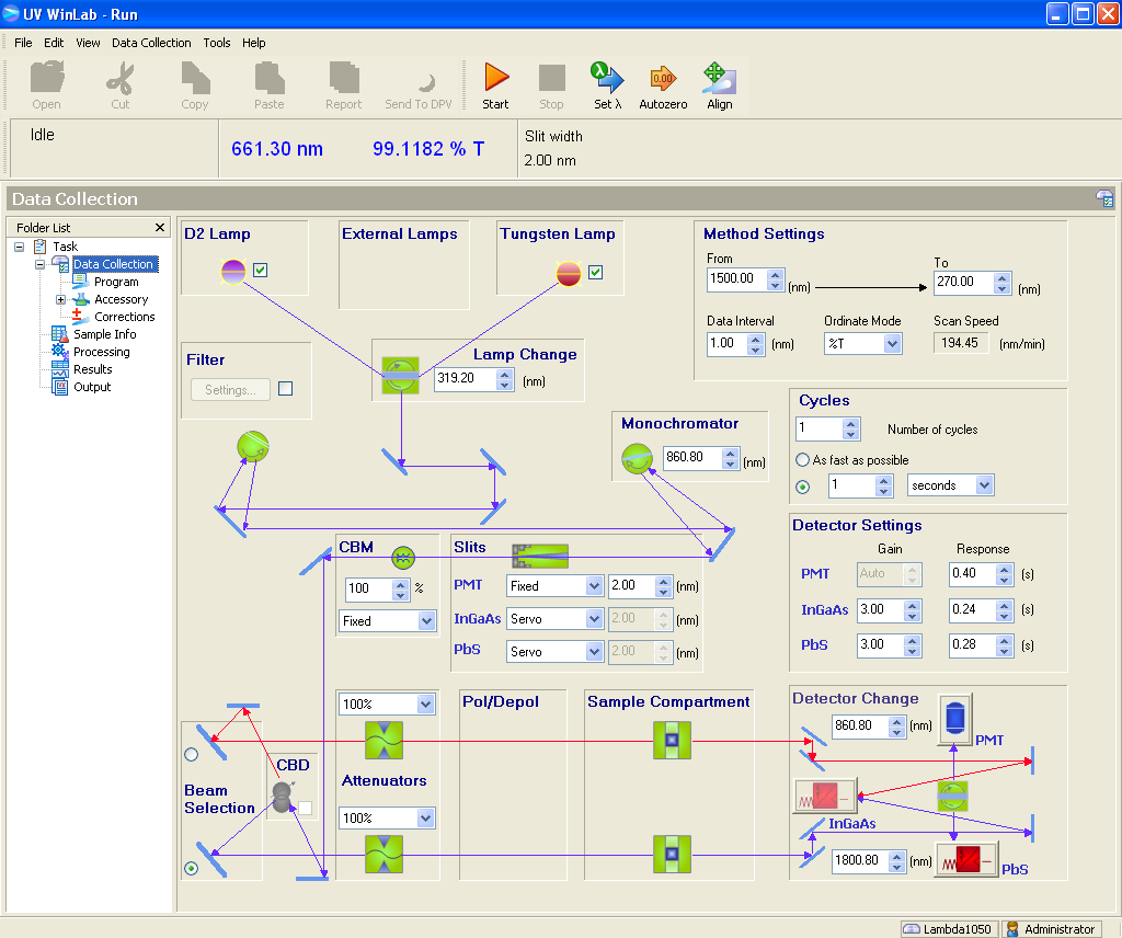
.sp files. The diagram follows the light, from the lamps at the top to the
sample compartment and the detectors at the bottom; the sample beam is purple, the
reference beam red. Screenshot of the PerkinElmer UV WinLab software.Almost the whole measurement is decided on this page. The values in the figure are the defaults, the same as in the three test files: range from 1500 to 270 nm with a 1 nm step, in %T; photomultiplier slit fixed at 2 nm and NIR slits on Servo; response times of 0.40 s (photomultiplier), 0.24 s (InGaAs) and 0.28 s (PbS); automatic gain for the photomultiplier and 3 for the NIR detectors; attenuators at 100 % on both beams; common beam mask at 100 %. They are fine up to absorbance 2–2.5, method A of the Procedures tab. With an ND100000, and with sun-viewing glasses, whose absorbance in the visible is between 4.5 and 6, they give nothing but noise over most of the spectrum: in the test files the transmittance of the ND100000 stays within the instrument's background throughout the ultraviolet and the visible, and between 875 and 1275 nm it is even negative, the mark of an offset rather than of a signal. The limit is not the instrument but the settings. The table says what to change, panel by panel, in the order in which it matters; the reason for each choice is in the Use tab, the complete measurement sequence in the Procedures tab.
| Panel | Default | ND100000 | Sun-viewing glasses | Why |
|---|---|---|---|---|
| Attenuators bottom left |
100 % and 100 % | upper menu (reference, red beam): 1 %, that is 2 A; 0.1 % (3 A) if the noise stays high. Lower menu (sample, purple beam): Automatic | as for the ND100000 | with the reference open the sample signal is a hundred thousand times weaker, and the ratio between the two suffers from noise and offset. The reference attenuation does not enter the result, because the baseline removes it; with Automatic the Autozero also collects the attenuator spectrum |
| Corrections in the list on the left |
100 %T only: the 0 %T was missing, as the negative readings show | also 0 %T / Blocked Beam Baseline, with Use internal attenuator | as for the ND100000 | it is the correction that removes the additive offset, the one behind the negative readings |
| Detector Settings right, middle |
PMT Auto and 0.40 s; InGaAs 3 and 0.24 s; PbS 3 and 0.28 s | PMT 2–5 s below 700 nm; InGaAs gain 6–10 and 1–2 s; PbS gain 1 | PMT 2–5 s up to 780 nm; in the infrared as for the ND100000 | the noise falls as \(1/\sqrt{t}\), up to 10 s per point, but only once the offset is gone. The NIR gain is what the application note calls sensitivity |
| Slits middle |
PMT Fixed 2.00 nm; InGaAs and PbS Servo | PMT Fixed 4–5 nm; NIR Servo or Fixed 3–5 nm | PMT 4–5 nm; NIR 5–10 nm or Servo | a neutral filter has no fine structure: a wide slit brings more energy and costs little in resolution. The maximum is 5 nm for the photomultiplier, 20 nm in the NIR |
| Method Settings top right |
From 1500, To 270, Data Interval 1, Ordinate Mode %T | From 2500, To 270; step 2–5 nm; A | From 2000 (better 2500), To 280; step 2–5 nm; A | at 1500 nm the transmittance of the ND is still rising, and the standard for the glasses goes up to 2000 nm. In absorbance high densities can be read, and the instrument noise is specified in A. Scan Speed is recalculated by itself: \(v = 60\,\Delta\lambda / t\) nm/min |
| Common Beam Mask middle left (CBM) |
100 %, Fixed | 100 % | 100 % if the aperture of the sample holder lies within the lens; less if the lens is lower than the beam | the beam is about 12 mm high: at absorbance 5 the light that passes beside the sample is worth more than the sample. The baseline must be taken with the same mask |
| Detector Change, Lamp Change, Monochromator |
860.8 and 1800.8 nm; 319.2 nm; 860.8 nm | unchanged, but with slit and time equal on both sides of 860.8 nm | with different parameters on the two sides a step appears: in the test files, for the ND100000, −113 % | |
| Cycles, Beam Selection, CBD |
1; front beam; off | unchanged: replicates are made as separate measurements, repositioning the sample, which goes in the holder of the purple beam | the depolariser is not needed for filters and films at normal incidence; if it is inserted, it must also be there for the baseline | |
For values that differ from one region to another, for instance long times below 700 nm and shorter ones in the infrared, choose Programmed in the Slits panel and fill in the Program page: the slits, times, NIR gains and attenuators of this page turn grey and are set there, row by row. Then: method saved under a new name, lamps on for at least an hour, light-tight sample holder with an aperture smaller than the sample, Autozero from the toolbar with the compartment empty and closed and the attenuators already in place, and finally Start. A fixed scale is advisable for the chart (in Graph Properties, from 0 to 8 A, without Autorange): with the automatic scale even noise looks like a spectrum. The bar under the commands shows the current wavelength and reading (661.30 nm and 99.1182 %T in the figure, with the compartment empty): with the sample beam closed it must drop close to zero. With a 5 nm step and 5 s per point, a scan from 2500 to 270 nm takes about 40 minutes.
A measurement, step by step
- Switch the instrument on, start UV WinLab, wait for the end of the initialisation and for the lamps to warm up.
- In the Explorer open a Scan method and save it at once with File › Save Settings › As New Method and a name that says what it is for: methods and tasks cannot be renamed, and a method changed but not saved produces a "one-off" task whose template is lost.
- Data Collection: range and step, ordinate mode, slits, response times, gains, attenuators. For parameters that differ by region, choose Programmed and fill in the Program page.
- Corrections: select 100 %T / 0A Baseline (Autozero) and, for dense samples, 0 %T / Blocked Beam Baseline with Use internal attenuator: the program closes the sample attenuator by itself to measure the dark signal. With Save Corrections the baselines stay attached to the method.
- Sample Info: the sample names, with position and orientation, because the file does not record them anywhere else.
- Autozero (Data Collection menu or toolbar) with the compartment empty and closed: it collects the selected corrections.
- Start: the program asks for the samples to be inserted and measures. The results
are saved in the task (Save Results); the spectra are saved as
.sp(Save Spectra, or Save as Binary from the chart menu) and exported as ASCII, JCAMP-DX or CSV (Export). The.spfiles are what this page reads.
Behaviours worth knowing
- Changing a Data Collection parameter invalidates the baselines, unless Do not invalidate baselines with respect to instrument settings is ticked; even with that option, a wider range or a finer step forces new ones.
- The frequency Always before next measurement means before every block of measurements, not before every sample.
- The header of a correction spectrum shows the current conditions, not those under which the correction was measured; with the automatic attenuator the status shows the sample setting, not the one actually used.
- Parameters must not be changed while the sample table is running.
- Methods saved with 6.0.4 cannot be imported into 6.0.3 unless exported with the compatibility option.
- A flat line at 100 %T means a saturated detector: reduce slit or gain.
Official sources
- PerkinElmer, UV WinLab Software Guide, version 6.0.4, November 2011, and UV WinLab Release Notes 6.0.4, from CD L6100139 Iss E: archive.org.
- PerkinElmer, High-Performance LAMBDA Spectrometers Hardware Guide, L6050008 A, December 2007, and Three Detector Module User's Guide, L6050010 A, December 2007 (copies published by a university teaching laboratory: pasta.place).
- PerkinElmer, Technical Specifications for the LAMBDA 1050 and LAMBDA 950, 008021_02, 2007: copy of the specification sheet.
- PerkinElmer, High Absorbance Scanning with the LAMBDA 850+ UV/Vis and LAMBDA 1050+ UV/Vis/NIR Spectrophotometers, application note: perkinelmer.widen.net.
What this utility is for
It reads .sp files without going through the instrument or its software and
derives from them everything needed to judge a transmittance measurement: the parameters it
was made with, the spectrum, the quantities of interest for a filter (photopic absorbance,
stops, maximum of the infrared transmission band, infrared fraction of the
transmitted energy) and, above all, how reliable the measurement is. This last point is
why the page exists: on a very dense filter the instrument writes a number in the file even
when that number is only its own background.
Step by step
- In the Input tab choose one or more files with the file field, or drag them onto the box. At most 50 files of 300 kB at a time: a 1231-point file weighs 11 kB.
- Analyse sends the files to the server in a single request; the computation takes
less than a second. Before decoding them the server checks that they really are
.spfiles (see File checks below): a damaged file, or one that is not an.sp, gets its own message and does not stop the others. - Each file has its own tab. The tab shows the file name and an icon that tells how it went: red if the file could not be read, yellow if the analysis left warnings; hovering over it shows the sample name. The tab contains the chart, the summary table and, collapsed under the table, the means over 100 nm blocks.
- Chart ordinate switches from linear transmittance to logarithmic scale and to absorbance without a new request, for all the files. In the last two only the points above the detection threshold are drawn (see below).
- Show together, available from two files up, puts all the spectra in a single chart above the tabs: one series per file, with different colours and line styles. A click on a legend entry switches the series off and another switches it back on; the legend can be dragged. The tabs remain, with only the tables, and here too no new request is needed.
- The bar above each chart saves the image as PNG, downloads the data as JSON and CSV (in the form shown: in absorbance, the absorbance), opens the customisation, the window zoom and the view reset.
An example: the three filters of the test files

This is what the page produces from the three .sp files of the technical
document: three photographic ND filters (ND64, ND1000 and ND100000) measured with the
LAMBDA 1050 between 1500 and 270 nm, with the default settings. To get there the program
checked each file before opening it, decoded its structure, rebuilt the wavelength axis and
estimated the instrument background for each detector; then it put the three transmittances
on the same logarithmic scale, which holds values from 10 % down to 0.001 %
together. What the chart shows:
- the three curves share the same spectral architecture, at different densities: cut-off between 360 and 400 nm, an almost flat course in the visible, a bulge between 700 and 860 nm, a minimum towards 1100 nm and a rise up to 1500 nm. They are filters of the same family;
- the dashed lines are the lamp change (319.2 nm) and the detector change (860.8 nm) recorded in the files: that is where to look for steps between one channel and the other;
- points below the detection threshold are not drawn, which is why the curves break off. Of the ND100000 only what rises above the background remains: the two infrared bands, between 680 and 860 nm and from about 1390 nm upwards, and a few isolated fragments where the noise crosses the threshold for a handful of points. In the visible its expected transmittance, 0.001 %, lies within the background of these settings: the table of its tab says so with "not measured", and the Instrumentation tab explains how to adjust the measurement.
File checks
The page is open to everyone, so the server treats every file as untrusted data: the
.sp extension is chosen by whoever uploads the file and proves nothing. Before
decoding a file it checks, in this order:
- the size: at most 300 kB per file and 50 files per request;
- the signature: the first four bytes must be
PEPE; - the type declared in the header: 2D constant interval DataSet file, the only one the page can read;
- the structure: the records, each with its identifier and its length, must cover the file exactly, with no missing or extra bytes, and be nested at most 16 levels deep.
During decoding, the number of points, the step and the end points of the abscissa must be valid, finite numbers, the data array must be made of 8-byte values and the ordinates must be plausible (within one million in absolute value); if the wavelengths fall outside the 100–5000 nm range the spectrum is shown, but the band quantities are not computed. A file that fails a check is not analysed, and the message in its tab says which check failed. No file is executed or kept: the server reads it from the request with a decoder written in Python, which uses neither external libraries nor the instrument software, and discards it at the end of the analysis.
How to read the table
- Sample and measurement, Instrument and method: what the file records about the state of the instrument. The labels with an asterisk are inferred from the content (Instrumentation tab). The date is that of the instrument PC's clock.
- Spectral data: range, step, extremes, number of negative readings — a negative transmittance is not physical, and their number is the first hint of an offset — and the consistency checks against the redundant fields of the file. A red check means a damaged file or a format different from the expected one.
- Derived quantities: every value has its standard error. When a quantity does not exceed the detection threshold the table does not give the number but a limit (< for transmittance, > for absorbance, stops and filter factor) and explains why.
- Measurement quality: for each detection channel the offset \(\delta\) and the background noise \(\sigma_0\), then the steps at the two changeovers. These are the numbers that tell whether the method used was suited to the sample.
The derived quantities
The photopic transmittance weights the spectrum with the CIE luminous efficiency function \(V(\lambda)\) and with a 5778 K black body, that is with sunlight as the eye sees it:
\[ T_v = \frac{\sum_{380}^{780} T(\lambda)\,V(\lambda)\,B(\lambda, 5778\ \mathrm{K})}{\sum_{380}^{780} V(\lambda)\,B(\lambda, 5778\ \mathrm{K})}, \qquad A = -\log_{10} T, \qquad \text{stops} = \log_2 \frac{1}{T} \]with \(T\) expressed as a fraction. The filter factor is \(1/T\); the red/blue imbalance is \(\log_2\) of the ratio between the 600–650 and 450–500 nm means; the energy fraction beyond 700 nm is computed over the measured range, and is therefore a lower bound if the spectrum stops before the transmittance drops. The luminous transmittance of ISO 12312-2 uses the D65 illuminant instead of the black body: the two do not coincide, although on a neutral filter the difference is small.
Noise, offset and detection threshold
The point-to-point noise is the standard deviation of the first differences divided by \(\sqrt{2}\), which removes the local slope; the standard error of a mean over \(n\) points is \(\sigma/\sqrt{n}\). A transmittance cannot be negative: a negative mean over a 100 nm block therefore measures an additive instrument error directly. The largest of them, for each detection channel (below and above the detector change: on the LAMBDA 1050 photomultiplier and InGaAs), is the offset \(\delta\). A transmittance \(T\) with standard error \(s\) is considered measured if
\[ T > 3\,\max(\delta,\ s) \]otherwise the table gives its upper limit \(\max(T, 0) + 3\max(\delta, s)\), and from it a lower limit of the absorbance. The same criterion applies to the charts on a logarithmic scale and in absorbance: only the points above \(3\max(\delta, \sigma_0)\) are drawn, with \(\sigma_0\) the background noise of the channel; a value that is positive but inside the noise would become a meaningless peak (absorbance 6 where the filter is merely opaque). A longer integration reduces \(s\), not \(\delta\): when the offset sets the limit, the measurement is improved with the 0 %T correction and the attenuation of the reference, not with more time.
At the changeover points (lamp change and detector change, read from the file) two straight lines are fitted over 31 nm on the left and on the right and the extrapolated values are compared: the transmittance of a sample does not jump exactly where the instrument changes detector, so the step measures the disagreement between the two channels.
Characterising an ND100000 filter

An ND100000 has a nominal absorbance of 5 (0.001 %T, 16.6 stops) in the visible and, as the files of the technical report show, transmits much more in the near infrared (absorbance 4.1–4.5 between 675 and 875 nm, 3.3 at 1500 nm, with the transmittance still rising). With the parameters of the test files — both attenuators at 100 %, response times of 0.24–0.4 s, no 0 %T correction — the visible reading is inside the background: the page reports it as "not measured" with photopic absorbance > 4.7. The parameters to act on, in order of importance:
| Parameter (UV WinLab) | What to do | Why |
|---|---|---|
| Rear beam attenuator (the rear beam is the reference, unless Beam Selection says otherwise) | 1 % (2 A) as a starting point for a 5 A sample; 0.1 % (3 A, 1050 only) if the noise stays high. No more than 4 A in total | with the reference open, the sample signal is a hundred thousand times weaker and their ratio, which the instrument alternates every 40 ms, suffers from noise and offset; attenuating the reference brings the two signals closer. It does not increase the absorbance of the sample: the baseline removes it |
| Front beam attenuator (sample) | Automatic | the program measures three spectra (100 %T, 0 %T and attenuator) and combines them: it recovers the signal-to-noise ratio where the sample transmits a lot, as in the infrared bands |
| Corrections › 0 %T / Blocked Beam Baseline | on, with Use internal attenuator | it is the correction that removes the additive offset responsible for the negative readings, i.e. the table's \(\delta\) |
| 100 %T / 0A Baseline (Autozero) | with the attenuators already in place, compartment closed, right before the measurements and with the same parameters | a baseline taken with parameters different from those of the measurement brings back the steps at the changeovers |
| Response time (PMT Response, InGaAs Response) | 1 s (application note), up to 2–5 s per point in the densest regions | the noise falls as \(1/\sqrt{t}\); it helps only after the offset has been removed |
| Step (Data Interval) and speed | 1–2 nm; 5 nm with long integrations | the maximum speed is \(v = 60\,\Delta\lambda / t\) nm/min: with 1 nm and 1 s about 30 nm/min, with 2 nm and 2 s about 60 |
| UV/Vis slit | 2–4 nm (application note); up to 5 nm | a neutral filter has no fine structure: a wide slit brings more energy and costs little in resolution |
| NIR slit and gain | servo or 3–5 nm; InGaAs gain 6–10 (1 for PbS) | the InGaAs channel is the one with the largest offset in the test files (0.002 %T) |
| Range | extended at least to 2500 nm (the wide-band InGaAs reaches it) | at 1500 nm the transmittance is still rising: it is the part of the spectrum where the absorbance of the filter falls |
| Common beam mask | 100 % | all the energy is needed |
| Warm-up | at least one hour before the baseline | the three test files show a zero drift of 0.0006 %T in 51 minutes |
After the measurement, the page tells whether it worked: \(\delta\) of both channels well below the level sought (0.001 %T for absorbance 5), the photopic transmittance "measured" with a standard error of the order of 0.0001 %T, the visible blocks classified as signal, a relative step at the detector change of a few percent. The complete sequence, with the validity checks, is in the Procedures tab.
Characterising sun-viewing glasses (ISO 12312-2)

ISO 12312-2:2015 covers filters for the direct observation of the Sun with the naked eye (glasses, viewers): it does not apply to filters for lenses, binoculars and telescopes. For transmittance it requires (table 1 of the standard, as reported by the American Astronomical Society and by its principal author, B. R. Chou):
| Quantity | Range | Requirement |
|---|---|---|
| luminous transmittance \(\tau_v\) (D65, \(V(\lambda)\)) | 380–780 nm | between 0.000061 % and 0.0032 %, i.e. absorbance between 6.21 and 4.49 (scale numbers 12 to 15) |
| solar UV-B transmittance \(\tau_{\mathrm{SUVB}}\) | 280–315 nm | not above \(\tau_v\) |
| solar UV-A transmittance \(\tau_{\mathrm{SUVA}}\) | 315–380 nm | not above \(\tau_v\) |
| solar IR transmittance \(\tau_{\mathrm{SIR}}\) | 780–2000 nm | not above 3 % |
The "solar" transmittances are averages weighted with the solar spectrum, not maxima at each wavelength; the standard also requires uniformity within 10 %, no defects outside a 5 mm margin (for metal-coated films, at most one 200 µm pinhole in any 5 mm diameter zone) and the warnings on the label. The test methods are those of ISO 12311:2013, now part of ISO 18526-2, -3 and -4 of 2020; a new edition of 12312-2 is being approved (FDIS, 2026). For the measurement four things matter:
- The range goes from 280 to 2000 nm: below 319.2 nm the deuterium lamp works, above 860.8 nm the InGaAs. In the ultraviolet the sample is very dense and the energy low: attenuators and times as for the ND100000.
- The lower limit coincides with the instrument's stray light: 0.000061 %T against the 0.00007 %T declared at 220–370 nm. Proving that a filter is not too dark is at the edge of what the LAMBDA 1050 can do; proving that it is not too light (0.0032 %, absorbance 4.5) is within its reach with the high-absorbance method.
- Uniformity: several positions per lens (at least three, away from the 5 mm margin) and both lenses. The beam is about 12 mm high: on small lenses the common beam mask reduces it, and the sample holder must have an aperture smaller than the lens and keep the film flat.
- What this page computes: photopic transmittance with the black body, absorbance, spectrum and measurement quality, but not yet \(\tau_v\) with D65 nor the weighted solar transmittances. Its job here is to tell whether the measurement holds up: whether the visible absorbance is "measured" and not a limit, whether the offset is below the level to be verified, whether the 780–2000 nm range is covered. The conformity calculation must be done with the tables of the standard.
What transmittance is
The International Lighting Vocabulary (CIE S 017) defines transmittance as the ratio of the transmitted to the incident radiant flux, \(\tau = \Phi_t / \Phi_i\). The transmitted flux has two parts: the one that continues in the direction of the beam (regular transmittance \(\tau_r\)) and the one scattered in other directions (diffuse transmittance \(\tau_d\)), with \(\tau = \tau_r + \tau_d\). A double-beam spectrophotometer without an integrating sphere measures the regular transmittance: for a good optical filter it is practically all of it, for a plastic film or a ground glass it is not.
Absorbance is \(A = -\log_{10}\tau\): a filter with \(A = 5\) transmits \(10^{-5}\), 0.001 %. It is the quantity UV WinLab calls "A". The CIE vocabulary lists it as transmittance optical density, with the synonyms optical density and decadic absorbance; IUPAC calls it absorbance and discourages the name optical density, which is however still common for photographic filters. Computed on the transmittance of the whole filter, as the instrument does, absorbance includes the reflection losses at the two surfaces. That of the material alone between the surfaces is the internal absorbance \(A_i = -\log_{10}\tau_i\), with \(\tau_i\) the internal transmittance: it is the quantity to which the CIE reserves the name spectral absorbance, defined for a homogeneous, non-diffusing layer. For a homogeneous material the internal absorbance grows linearly with the thickness and with the concentration of the absorbing species (Bouguer-Lambert-Beer law):
\[ A_i = \varepsilon\, c\, \ell, \qquad \tau_i = 10^{-A_i} \]with \(\varepsilon\) the molar absorption coefficient, \(c\) the concentration and \(\ell\) the optical path. The law holds for monochromatic light, homogeneous and non-scattering samples, and has precise optical limits (interference in thin films, multiple reflections) that make it an approximation even when the chemistry is ideal. A metal-film ND filter does not follow Lambert-Beer at all: its absorbance comes from reflection and absorption in a layer of fixed thickness.
Photographic filters use the stop, a halving of the light: \(\text{stop} = \log_2(1/\tau) = A / \log_{10}2 \approx 3.32\,A\). An ND1000 has absorbance 3, i.e. 10 stops; an ND100000 absorbance 5, 16.6 stops. Protective filters use the scale number \(N = 1 + \tfrac{7}{3}\log_{10}(1/\tau_v)\): a luminous absorbance of 5 corresponds to \(N \approx 12.7\).
How a double-beam spectrophotometer works
The instrument answers a simple question — what fraction of the light passes at each wavelength — with three solutions, each against a source of error.
The monochromator isolates a narrow band of wavelengths: a diffraction grating disperses the light, an exit slit lets through a slice of width \(\Delta\lambda\) (the bandwidth, set by the slit). The enemy is stray light, radiation of other wavelengths that reaches the detector by scattering on grating, mirrors and walls. If \(s\) is the stray light fraction, the instrument reads
\[ T_{\text{read}} = \frac{T + s}{1 + s} \;\approx\; T + s \quad\text{for } T \ll 1 \]and below \(T \approx s\) it can no longer tell anything apart: with \(s = 7\cdot10^{-7}\) (the declared 0.00007 %) the ceiling is an absorbance of 6.2. A double monochromator, two monochromators in series, brings the stray light to values of the order of the product of the two: this is what makes it possible to measure filters at absorbance 5–6. Holographic gratings, made by interference rather than by mechanical ruling, have fewer periodic defects and hence less stray light and fewer ghost lines.
The double beam compares the sample with a reference measured almost at the same instant. The chopper alternates, more than 46 times a second, dark, sample beam, dark, reference beam; the detector is the same, and the ratio of the two beams cancels the slow variations of lamp, detector and electronics. UV WinLab then corrects the ratio with two baselines measured before the samples, \(B_{100}\) with the compartment empty and \(B_0\) with the beam blocked; the guide describes the correction with these quantities, in the usual form
\[ T = 100\,\% \cdot \frac{T_{\text{raw}} - B_0}{B_{100} - B_0} \]This is the 0 %T correction missing from the test files: without \(B_0\), an additive error of the electronics stays in the result and, on an almost opaque sample, becomes a negative transmittance.
The dynamic range is the least intuitive limit. With a sample at absorbance 5 the detector receives a signal a hundred thousand times weaker on the sample beam than on the reference beam, and switches from one to the other every 40 ms: the gain, set on the reference, stays low, and the sample signal ends up in the zone where offset and noise of the electronics are comparable to it. The UV WinLab guide explains it this way, and the cure is to attenuate the reference by a known factor (10 %, 1 %, 0.1 %), which the baseline then removes.
The sources
No single lamp covers 175 to 3300 nm. The deuterium lamp is a gas discharge that emits a continuum in the ultraviolet, from about 160 to 400 nm, with a few narrow lines in the visible (486.0 and 656.1 nm) used to check the wavelength scale. The tungsten-halogen lamp is an incandescent filament, almost a black body at about 3000 K, emitting from about 340 nm to beyond 3000 nm. The instrument switches from one to the other where both are weak, by default at 319.2 nm. The consequences can be seen in the files: below 420 nm the halogen lamp has little energy, and the 400–500 nm band is the noisiest in relative terms; at the lamp change there is a small step. The lamps must warm up: the hardware guide says about one hour, and the test files show a drift still in progress.
The detectors
- Photomultiplier (175–860 nm). The multi-alkali photocathode emits electrons by the photoelectric effect, a chain of dynodes multiplies them millions of times: very high sensitivity and low noise in the ultraviolet and visible. Beyond 850 nm the sensitivity of the photocathode collapses.
- InGaAs (860–1800 or 860–2500 nm). A semiconductor photodiode: the standard compound has a band gap of 0.73 eV and responds up to 1.7 µm; the "extended" or wide-band versions reach 2.5 µm at the price of a higher dark current, and are therefore cooled with Peltier cells.
- Lead sulphide (up to 3300 nm). A photoconductor, the first practical infrared detector in history: slow, noisy, temperature-sensitive, it works well only with modulated light — the chopper — and cooled.
Every detector change is a delicate point. On each side work detectors with different sensitivity, gain, noise and dark current, often with different slits: if the baseline was not taken with the same parameters, or if an additive error weighs differently on the two channels, the spectrum has a step. In the test files the step at 860.8 nm is −2 % on the ND64, −8.5 % on the ND1000 and −113 % on the ND100000: it grows as the signal decreases, the signature of an additive error. Near 860 nm the InGaAs is also at the edge of its band, where the sensitivity is only just rising.
The problems of the measurement
| Problem | Effect | Remedy |
|---|---|---|
| stray light | ceiling on the measurable absorbance (A ≈ 6.2 for this instrument); readings too high, never negative | cannot be worked around with the settings: it is the instrument's specification |
| offset and dark current | additive error; negative readings on opaque samples | 0 %T correction, reference attenuation |
| drift | zero moving with time | warm-up, close baselines, final dark check |
| noise | point-to-point scatter | integration time, slit, averaging of several scans: scales as \(1/\sqrt{t}\) |
| bandwidth | smooths narrow structures; almost irrelevant on a neutral filter | slit suited to the sample |
| polarisation | gratings and mirrors polarise; on tilted or birefringent samples the reading depends on orientation | common beam depolariser, normal incidence |
| multiple reflections | light bouncing between sample and optics; beam shift with thick or tilted samples | normal incidence, sample close to the detector, same position for baseline and measurement |
| sample inhomogeneity | the result depends on the point crossed | several positions, aperture, recorded orientation |
| thin films | interference fringes, structure that shifts with the angle of incidence | normal incidence; the fringes give the thickness (below) |
| scattering by the sample | regular transmittance underestimates the total one | integrating sphere, if total light matters |
The problems of the software
UV WinLab is the only way to drive the instrument, and it brings four kinds of problems with it.
It is proprietary and closed. It has no documented programming interface: every
measurement goes through the graphical interface. The data sit in an encrypted Access
database, and the .sp format in which they come out is not published — what the
Instrumentation tab describes was reconstructed. A laboratory that wants its own data
in an open form has to export them, file by file, as ASCII or CSV, or use a tool such as this
page.
It is dated. 6.0.3 is a 32-bit program of the 6.0 generation (the 6.0.4 guide dates from November 2011), certified for Windows XP and Vista SP1: systems out of support for years, receiving no security updates. The instrument PC must therefore be kept off the network, data must be taken away on controlled media, and a complete image of the disk is worth keeping: if that PC breaks, a new PC may not be able to replace it.
The interface is unfortunate. The parameters of a measurement are scattered over several pages (Data Collection, Program, Corrections, Sample Info); the per-region ones are only visible row by row, and end up in the file as compact strings that no manual explains. The program invalidates the baselines when a parameter changes, but the header of a correction shows the current conditions and not those it was measured with; with the automatic attenuator the status shows the setting and not the value used. Methods and tasks cannot be renamed, a method changed and not saved produces a result whose template is lost, a method opened during the initialisation may freeze. None of this prevents a good measurement, but it makes it easy to make a bad one without noticing — which is what happened with the test files, measured with a method never re-optimised for those samples.
The connection belongs to another era. The LAMBDA 1050 of this generation talks over a 25-pin RS-232 serial line. Modern PCs have no serial ports: a native serial card (PCI or PCIe) or a USB adapter is needed, which no official document accepts, and cheap converters have timings and drivers that a program written for real serial ports does not expect. The 6.0.4 release notes fix precisely a serial-port defect of 6.0.3 (time-drive acquisitions with intervals beyond 40 s failed because of a timeout). Newer models have a USB port, but require UV WinLab 6.3 or later, and Windows 10 requires 6.4/6.5 (sold as a separate upgrade, on top of 6.0.4) or 7. Upgrading therefore means changing program version and revalidating the methods: those saved with 6.0.4 do not go back into 6.0.3 except through a dedicated export.
What else can be measured with this instrument
- Absorbance and concentration of solutions in a cuvette, with the Lambert-Beer law and the calibration curves of the quantitative methods.
- Specular reflectance with the reflectance accessories, also as a function of angle (the universal accessory URA and the TAMS system measure absolute transmittance and reflectance at several angles).
- Total and diffuse reflectance and transmittance with the 150 mm integrating sphere, and from them the haze of transparent materials (ASTM D1003).
- Colour: chromaticity coordinates and luminous transmittance with any CIE illuminant and observer (CIE 015), starting from the spectrum.
- Optical band gap of semiconductors and films, from the Tauc plot.
- Thickness and refractive index of thin films from the interference fringes: two adjacent maxima at \(\lambda_1\) and \(\lambda_2\) give \(n d = \lambda_1\lambda_2 / [2(\lambda_2-\lambda_1)]\). From the ND64 maxima at 465 and 556 nm one gets \(n d \approx 1.42\) µm, the hint that it is a thin-film filter.
- Transmittance in polarised light, with motorised polariser and depolariser.
- Kinetics (Timedrive) and fixed-wavelength programs (Wavelength Program): the latter are the way to integrate for a long time on a few points, as the densest filters require.
Bibliography
- CIE S 017/E:2020, ILV: International Lighting Vocabulary, 2nd ed., DOI 10.25039/S017.2020 (entries 17-24-064, -065, -067, -069, -072, -088, -090).
- CIE 015:2018, Colorimetry, 4th ed., DOI 10.25039/TR.015.2018.
- CIE 130-1998, Practical Methods for the Measurement of Reflectance and Transmittance, DOI 10.25039/TR.130.1998.
- J. W. Verhoeven, "Glossary of terms used in photochemistry (IUPAC Recommendations 1996)", Pure Appl. Chem. 68, 2223 (1996), DOI 10.1351/pac199668122223 (entry optical density, p. 2257).
- T. G. Mayerhöfer, S. Pahlow, J. Popp, "The Bouguer-Beer-Lambert Law: Shining Light on the Obscure", ChemPhysChem 21, 2029 (2020), DOI 10.1002/cphc.202000464.
- T. A. Germer, J. C. Zwinkels, B. K. Tsai (eds.), Spectrophotometry: Accurate Measurement of Optical Properties of Materials, Academic Press, 2014, ISBN 978-0-12-386022-4.
- R. Mavrodineanu, J. I. Shultz, O. Menis (eds.), Accuracy in Spectrophotometry and Luminescence Measurements, NBS SP 378 (1973), DOI 10.6028/NBS.SP.378.
- K. D. Mielenz, "Physical parameters in high-accuracy spectrophotometry", J. Res. NBS 76A, 455 (1972), DOI 10.6028/jres.076A.040.
- K. D. Mielenz, K. L. Eckerle, "Spectrophotometer linearity testing using the double-aperture method", Appl. Opt. 11, 2294 (1972), DOI 10.1364/AO.11.002294.
- K. D. Mielenz, R. Mavrodineanu, "Reflection correction for high accuracy transmittance measurements on filter glasses", J. Res. NBS 77A, 699 (1973), DOI 10.6028/jres.077A.041.
- ASTM E387-04(2022), Estimating Stray Radiant Power Ratio of Dispersive Spectrophotometers by the Opaque Filter Method, DOI 10.1520/E0387-04R22.
- W. Kaye, "Stray light ratio measurements", Anal. Chem. 53, 2201 (1981), DOI 10.1021/ac00237a013.
- M. R. Sharpe, "Stray light in UV-VIS spectrophotometers", Anal. Chem. 56, 339A (1984), DOI 10.1021/ac00266a003.
- A. C. Hardy, "A new recording spectrophotometer", JOSA 25, 305 (1935), DOI 10.1364/JOSA.25.000305.
- H. H. Cary, A. O. Beckman, "A quartz photoelectric spectrophotometer", JOSA 31, 682 (1941), DOI 10.1364/JOSA.31.000682.
- A. Labeyrie, J. Flamand, "Spectrographic performance of holographically made diffraction gratings", Opt. Commun. 1, 5 (1969), DOI 10.1016/0030-4018(69)90068-6.
- R. D. Saunders, W. R. Ott, J. M. Bridges, "Spectral irradiance standard for the ultraviolet: the deuterium lamp", Appl. Opt. 17, 593 (1978), DOI 10.1364/AO.17.000593.
- Hamamatsu Photonics, Photomultiplier Tubes: Basics and Applications, 4th ed., 2017: hamamatsu.com.
- T. P. Pearsall, "Ga0.47In0.53As: a ternary semiconductor for photodetector applications", IEEE J. Quantum Electron. 16, 709 (1980), DOI 10.1109/JQE.1980.1070557.
- A. Rogalski, "History of infrared detectors", Opto-Electron. Rev. 20, 279 (2012), DOI 10.2478/s11772-012-0037-7.
- D. G. Goebel, "Generalized integrating-sphere theory", Appl. Opt. 6, 125 (1967), DOI 10.1364/AO.6.000125.
- ASTM D1003-21, Haze and Luminous Transmittance of Transparent Plastics, DOI 10.1520/D1003-21.
- P. Makuła, M. Pacia, W. Macyk, "How to correctly determine the band gap energy of modified semiconductor photocatalysts based on UV-Vis spectra", J. Phys. Chem. Lett. 9, 6814 (2018), DOI 10.1021/acs.jpclett.8b02892.
- R. Swanepoel, "Determination of the thickness and optical constants of amorphous silicon", J. Phys. E 16, 1214 (1983), DOI 10.1088/0022-3735/16/12/023.
- Z. M. Zhang, T. R. Gentile, A. L. Migdall, R. U. Datla, "Transmittance measurements for filters of optical density between one and ten", Appl. Opt. 36, 8889 (1997), DOI 10.1364/AO.36.008889.
- M. Lequime, S. Liukaityte, M. Zerrad, C. Amra, "Ultra-wide-range measurements of thin-film filter optical density over the visible and near-infrared spectrum", Opt. Express 23, 26863 (2015), DOI 10.1364/OE.23.026863.
- M. Comelli, Caratterizzazione spettrofotometrica di filtri a densità neutra (spectrophotometric characterisation of neutral density filters), CNR-IFAC technical report, 31 August 2026.
What a measurement procedure is
A UV WinLab method sets the parameters of the instrument, but does not say in which order things are done, with which checks, and when the result is accepted. A procedure has five parts, to be written before sitting down at the instrument:
- the aim: which quantity, over which range, with which uncertainty (for a solar filter: the absorbance in the visible, the transmittance in the ultraviolet and in the infrared, with an uncertainty that allows the comparison with the limits);
- the methods: the parameters of the instrument, region by region, saved with names that say what they are for;
- the sequence: preparation, corrections, control measurements, samples, replicates, final checks;
- the acceptance criteria: the numbers the measurement must meet to be kept — this page computes them;
- the record: what the
.spfile does not record.
The three methods
The choice depends on the absorbance expected in the region, not on the sample: the same filter may need one method in the visible and another in the bands where it transmits more.
| Method | Absorbance | Settings |
|---|---|---|
| A — standard | 0–2.5 | attenuators at 100 %; UV/Vis slit 2 nm, NIR servo or 2–3 nm; response time 0.2–1 s; step 1 nm; 100 %T correction |
| B — medium absorbance | 2.5–4.5 | reference 1 % (2 A), sample Automatic; UV/Vis slit 2–4 nm; 1–2 s; step 1–2 nm; 100 %T and 0 %T corrections |
| C — high absorbance | 4.5–6 | reference 1 % for a 5 A sample, 0.1 % (3 A, internal on the 1050) or 1 % plus a magnetic screen from kit L1160560 for 6–7 A, without exceeding 4 A in total; sample Automatic; UV/Vis slit 4–5 nm, NIR 5–10 nm or servo; 2–5 s; step 2–5 nm; 100 %T and 0 %T corrections |
PerkinElmer's application note gives as starting levels: reference at 1 % for a 5 A sample; at 1 % plus the 6 % screen (1–1.5 A) for 6 A; at 1 % plus the 1 % screen (2 A) for 7 A. If non-linearity or artefacts appear, attenuate slightly less; the UV WinLab guide suggests considering the attenuators above 3 A and recommends them above 4 A. Kit L1160560 contains five screens, of 32, 14, 6, 4 and 1 %T. Above 6 A the limit is stray light: no attenuation moves it.
Common preparation
- Lamps on for at least one hour (better two for the densest samples); compartment clean and closed.
- Methods A, B and C saved with explicit names (for example
ND_B_270-2500), common beam mask at 100 %, no smoothing. - Light-tight sample holder, with an aperture smaller than the clear aperture of the filter: at absorbance 5 a single gap at the edge gives more signal than the sample, and shows up as a transmittance that is too high.
- Corrections with the attenuators, internal and external, already in place: 0 %T and 100 %T with the compartment empty, right before the series. From then on the attenuators are not touched.
- A scan with the sample beam blocked using the same method: it measures the background of the instrument, and is the reference against which the readings of the densest samples are compared. Loaded into this page it must give readings compatible with zero.
ND64 filter (A ≈ 1.8)
- Method A over the whole range, 250–2500 nm: with absorbance 1.8 in the visible and less than 1 in the infrared, attenuating the reference would make the result worse.
- To check on this page: \(\delta\) close to zero in both channels, relative step at the detector change within 1 % (in the test files, with different slits on the two sides, it is −2 %).
- Expected, from the test files: photopic absorbance 1.864, i.e. 6.2 stops.
ND1000 filter (A ≈ 3)
- Method B in the visible and ultraviolet (above 3 A the guide suggests considering the attenuators); method A is enough in the infrared bands, where the absorbance falls to 2–2.7.
- To check: offset of the photomultiplier channel below 5 % of the visible transmittance (0.005 %T), relative step within 2 %.
- Expected: photopic absorbance 3.03, i.e. 10.1 stops.
ND100000 filter (A ≈ 5)
- Method C in the ultraviolet and visible (270–700 nm); method B in the infrared bands (700–2500 nm), where the absorbance falls to 3.3–4.5. The two scans overlap by 40–50 nm to check that they agree.
- Sequence: blocked beam, ND100000, ND1000, ND64, ND100000 again, blocked beam. The second measurement of the ND100000 and the second blocked-beam scan give repeatability and drift.
- Reposition the filter (for example rotating it by 90°) and repeat: the difference estimates the homogeneity.
- To check: \(\delta\) of both channels below 0.0003 %T; photopic transmittance "measured" with a standard error of the order of 0.0001 %T; visible blocks classified as signal; relative step at the detector change within a few percent. If the photopic value stays a limit, the method is not yet good enough: lengthen the times or move to a fixed-wavelength program (15–20 wavelengths, 60–300 s each).
Sun-viewing glasses (ISO 12312-2)
- Range 280–2000 nm, better up to 2500. Method C from 280 to 780 nm (the expected absorbance in the visible is between 4.5 and 6.2); in the infrared the method is chosen according to the level: metal-coated films also attenuate the infrared, other materials may transmit much more of it.
- Mounting: the lenses are often thin, flexible films. They must be kept flat, without tension, perpendicular to the beam, with an aperture smaller than the lens and away from the 5 mm margin. If the lens is small, the common beam mask reduces the height of the beam (12 mm when fully open).
- Positions: at least three per lens, on both lenses; the standard requires uniformity within 10 %.
- Visual inspection, outside the instrument, for pinholes and defects: the standard allows at most one 200 µm pinhole in any 5 mm diameter zone. A pinhole crossed by the beam biases the measurement upwards.
- To check on this page, bearing in mind that the two limits of the standard are not proven in the same way. That the filter is not too light (\(\tau_v \le\) 0.0032 %) is proven even by a limit: if the page reports "< 0.0010 %", the requirement is met. That it is not too dark (\(\tau_v \ge\) 0.000061 %) requires instead a measured value, i.e. \(\delta\) below 0.00002 %T: this is at the declared stray light, and with this instrument a filter with an absorbance above 6 cannot be told apart from one at absorbance 6. Then, that the spectrum covers 780–2000 nm.
- Conformity: \(\tau_v\) with D65 and \(V(\lambda)\), and the solar UV-A, UV-B and IR transmittances, are computed with the tables of the standard from the exported spectra; the page does not do it yet.
Record
The .sp file does not record the method name, the screens added on the reference
beam, the scan speed, the number of cycles, the position and orientation of the sample, the
warm-up time. All this goes into a log kept next to the files, and the file name should
already say the essentials, for example ND100000_pos2_metC_20260930.sp. Keep both
the .sp and the ASCII export: the former carries the parameters, the latter can
be read without special tools.
Validation
| Check | How | Criterion |
|---|---|---|
| instrument background | scan with the sample beam blocked | readings compatible with zero, without structure; on this page \(\delta\) and negative readings almost nil |
| additivity | ND64 and ND1000 stacked | absorbance of the stack equal to the sum of the two, within the uncertainty: in the visible about 1.870 + 3.005 = 4.875. It is the check at the absorbance level of interest, and needs no certified samples |
| substitution | the ND1000 already measured in the reference beam, the ND100000 in the sample beam | \(A_{100000} = A_{\text{read}} + A_{1000}\) must agree with method C within the quadrature sum of the uncertainties |
| repeatability | three replicates with repositioning | the scatter estimates together the repeatability of the instrument and the inhomogeneity of the sample |
| photometric scale | certified reference filters: NIST SRM 2031 (10, 30 and 90 %T) is still produced, the 1930 and 2930 series (down to 0.1 %T) no longer | checks the scale, but only up to absorbance 1–3: higher up, additivity and substitution remain |
The logic of substitution and of the reference cascade is that of high-absorbance metrology (Zhang et al., Appl. Opt. 36, 8889, 1997); the additivity check is that of Agilent note 5991-2528EN on the Cary 7000. The attenuator settings come from PerkinElmer's application note and from the UV WinLab guide (Instrumentation tab).
Keywords: spectrophotometer, transmittance, absorbance, PerkinElmer, UV WinLab, LAMBDA 1050, .sp, ND filter, neutral density, ND100000, photopic, V(λ), ISO 12312-2, eclipse glasses, solar filters, offset, noise, stray light, attenuators, detector change, RS-232, gw2py